Getting started

Let’s say you want to study a EPR cw spectrum, first you will like to load the data and see, what are it’s resonant fields and the peak to peak distance (Hpp). To do that process you can use the epraya.Seek function by calling

>>> import epraya as epr
>>> B,spc=epr.Seek()

This will open a new window (like the one below), where you can see the spectrum, its first and second integral and the base line options. This base line is defined adjust the spectrum with x axis and be comparable with the simulations.

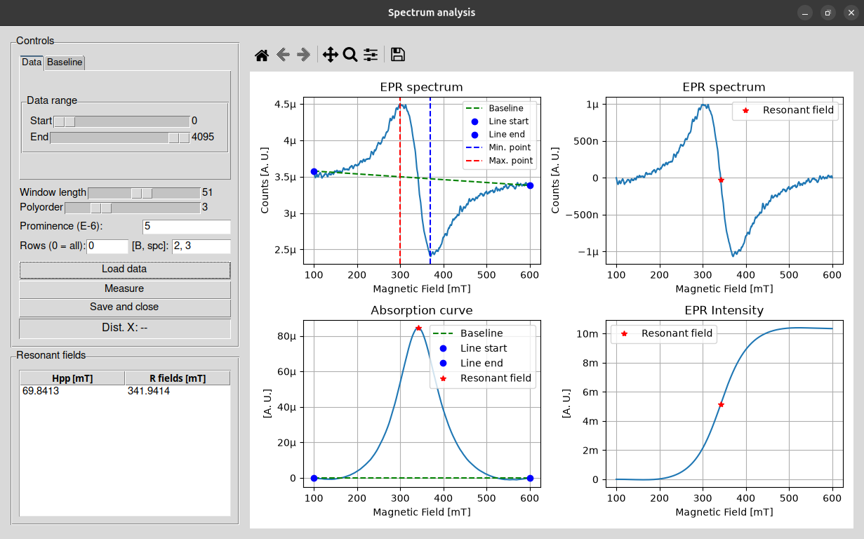
Other variables are the window lenght and the polyorder (polynomial order) of the Savitzky–Golay filter that is applied to the data, the prominence of the peaks in the first integral, use as reference to find the resonant fields.

After loading the data and filtred the spectrum, it may be a good idea to compare it with the theoretical one. To do this, you might know some properties of the spin system, for example, that it has a electronic spin of 3/2, a g factor of 2.003 and (from the Seek function) a peak to peak distance of around 70 mT.

Because you make the measurement also know that the sample was in powder form, that you take 4096 points from 100 mT to 600 mT, that the frecuency of the radiation was 9.43 GHz and the sample was at 80 K. With that information, using the containers Ham and Exp, for the hamiltonian and experimental information, respectly, you can simulate the theorical spectrum using the epraya.Powder like this:

>>> import epraya as epr
>>> Ham, Exp, Vary = epr.Start()
>>> Ham.S = 3/2
>>> Ham.g = [2.003,2.003,2.003]
>>> Ham.Hpp = [0, 70]
>>> Exp.Points = 4096
>>> Exp.Freq = 9.43
>>> Exp.Frange = [100,600]
>>> Exp.Temperature = 80
>>> B1,spc1 = epr.Powder(Ham,Exp)

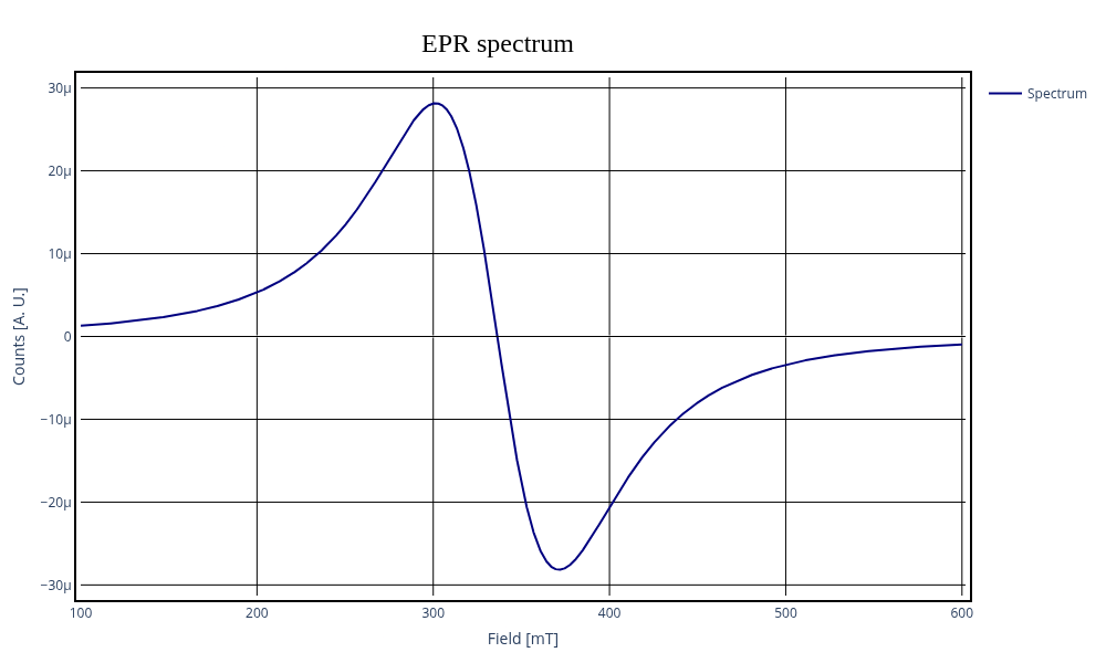
Having both simulated and experimental spectrums, they won’t match in general (of course), so you might have to fit the parameters using some method. In this case, you can use the implemented functions Nelder-Mead, Genetic algorithm, Metropolis and Least squares, calling them directly or using the wrap function epraya.Fitting.

But, how do you vary the values? This is where the container Vary is relevant for the process. It follows the same logic of the Ham, however saves the ranges to change the parameters. For example, if you want to change the g factor to fit the data, it will be:

>>> Vary.g=[1.5,2.5,1.5,2.5,1.5,2.5]
>>> epr.Fitting(Ham,Exp,Vary,spc)

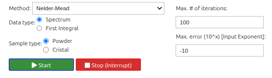
After starting the process and finding the values that correspond to the experimental data, you can make other analysis of the data, like seeing the temperature variation with epraya.Termal, the angle dependance epraya.Nrotate or more, using the functions in the Special functions category.

The JAX alternative

The EPRAYA package comes with a implementation in the JAX proyect to take advantage of GPUs speed in calculations. The structure is the same that the one described above, but with a change in the names of the functions (added a J):

>>> import epraya as epr
>>> Ham, Exp, Vary = epr.Jstart()
>>> Ham.S = 3/2
>>> Ham.g = [2.003,2.003,2.003]
>>> Ham.Hpp = [0, 70]
>>> Exp.Points = 4096
>>> Exp.Freq = 9.43
>>> Exp.Frange = [100,600]
>>> Exp.Temperature = 80
>>> B1,spc1 = epr.JPowder(Ham,Exp)

In the current version, none of the fitting functions are implemented with JAX, except for a ADAM algorithm implementation epraya.Briggs. For more details and how to use, see Jax implementation.